Circuit-based quantum programming
This is the training session for the preliminary understanding about QLM language

Usage
Creating a bell pair
 1from qat.lang import Program, H, CNOT, X, S
 2
 3# Create a Program
 4qprog = Program()
 5nbqbits = 2
 6qbits = qprog.qalloc(nbqbits)
 7
 8H(qbits[0])
 9CNOT(qbits[0], qbits[1])
10
11# Export this program into a quantum circuit
12circuit = qprog.to_circ()
13circuit.display()
14
15# Import a Quantum Processor Unit Factory (the default one)
16from qlmaas.qpus import get_default_qpu
17# from qlmaas.qpus import get_default_qpu to run on the QAPTIVA appliance
18qpu = get_default_qpu()
19
20# Create a job
21job = circuit.to_job(nbshots=100)
22result = qpu.submit(job)
23
24# Iterate over the final state vector to get all final components
25for sample in result:
26    print("State %s amplitude %s, %s (%s)" % (sample.state, sample.amplitude, sample.probability, sample.err))
Result
1State |00> amplitude None, 0.48 (0.05021167315686783)
2State |11> amplitude None, 0.52 (0.05021167315686783)
More advanced features:
nbshotsin job- Measure only certain qubits
- Difference between
sample.amplitudeandsample.probability - Difference between final measure and intermediate measure
Intermediate measurements
 1qprog = Program()
 2nbqbits = 2
 3qbits = qprog.qalloc(nbqbits)
 4H(qbits[0])
 5qprog.measure(qbits[0])
 6CNOT(qbits)
 7circuit = qprog.to_circ()
 8circuit.display()
 9
10
11qpu = get_default_qpu()
12job = circuit.to_job(nbshots=5, aggregate_data=False)
13result = qpu.submit(job)
14
15for sample in result:
16    print(sample.state, sample.intermediate_measurements)

Result
1|11> [IntermediateMeasurement(cbits=[True], gate_pos=1, probability=0.4999999999999999)]
2|00> [IntermediateMeasurement(cbits=[False], gate_pos=1, probability=0.4999999999999999)]
3|00> [IntermediateMeasurement(cbits=[False], gate_pos=1, probability=0.4999999999999999)]
4|11> [IntermediateMeasurement(cbits=[True], gate_pos=1, probability=0.4999999999999999)]
5|11> [IntermediateMeasurement(cbits=[True], gate_pos=1, probability=0.4999999999999999)]
Useful tools for gates
You can check all the gates avalable in the myQLM demo: Open Available Gates Tutorial. You can also create personal gates
Quantum routines
 1from qat.lang.AQASM import Program, QRoutine, H, CNOT
 2
 3routine = QRoutine()
 4routine.apply(H, 0)
 5routine.apply(CNOT, 0, 1)
 6
 7prog = Program()
 8qbits = prog.qalloc(4)
 9for _ in range(3):
10    for bl in range(2):
11        prog.apply(routine, qbits[2*bl:2*bl+2])
12prog.apply(routine, qbits[0], qbits[2])
13circ = prog.to_circ()
14circ.display()
1circ = prog.to_circ(box_routines=True)
2circ.display()

Using typed registers
 1## quantum adder
 2from qat.lang.AQASM.classarith import add
 3prog = Program()
 4reg_a = prog.qalloc(2, QInt)
 5reg_b = prog.qalloc(2, QInt)
 6
 7X(reg_a[0])
 8X(reg_b[1])
 9
10# |a> = |10> ("2") and |b>=|01> ("1")
11# expect |a+b>|b> = |11>|01>
12prog.apply(add(2, 2), reg_a, reg_b)
13circ = prog.to_circ(inline=False)
14circ.display()
15
16
17qpu = get_default_qpu()
18result = qpu.submit(circ.to_job())
19for sample in result:
20    print(sample.state, sample.amplitude)

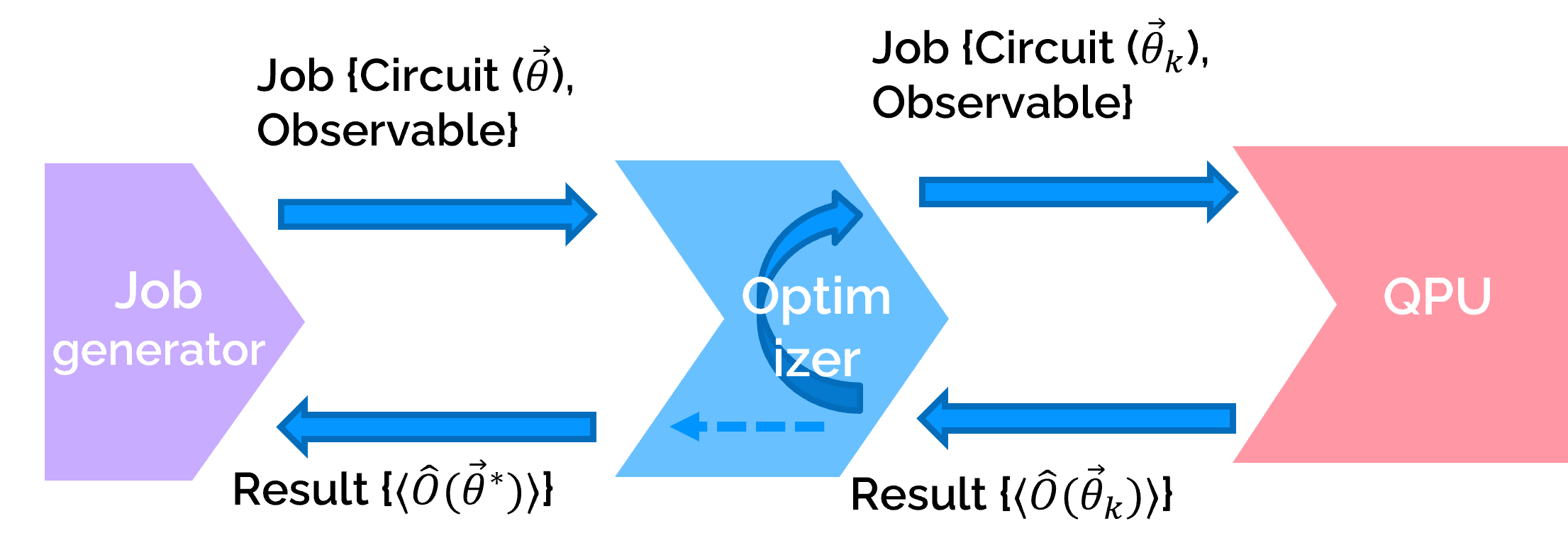
Variational computations
framework: Variational Quantum Eigensolver (VQE) is to find eigenvalues of a Hamiltonian
Our task: VQE on the following Ising model:
$$ H = \sum_{i=1}^{N} a_i X_i + \sum_{i=1}^{N} \sum_{j=1}^{i-1} J_{ij} Z_i Z_j $$… with a “hardware-efficient” ansatz.
 1import numpy as np
 2from qat.core import Observable, Term
 3
 4def ising(N):
 5    np.random.seed(123)
 6
 7    terms = []
 8
 9    # Generate random coefficients for the transverse field term (X)
10    a_coefficients = np.random.random(N)
11    for i in range(N):
12        term = Term(coefficient=a_coefficients[i], pauli_op="X", qbits=[i])
13        terms.append(term)
14
15    # Generate random coefficients for the interaction term (ZZ)
16    J_coefficients = np.random.random((N, N))
17    for i in range(N):
18        for j in range(i):
19            if i != j:  # avoid duplicate terms
20                term = Term(coefficient=J_coefficients[i, j], pauli_op="ZZ", qbits=[i, j])
21                terms.append(term)
22    ising = Observable(N, pauli_terms=terms, constant_coeff=0.0)
23    return ising
If we have the number of qubit = 4
1nqbits = 4
2model = ising(nqbits)
3print(model)
Result
 10.6964691855978616 * (X|[0]) +
 20.28613933495037946 * (X|[1]) +
 30.2268514535642031 * (X|[2]) +
 40.5513147690828912 * (X|[3]) +
 50.48093190148436094 * (ZZ|[1, 0]) +
 60.4385722446796244 * (ZZ|[2, 0]) +
 70.05967789660956835 * (ZZ|[2, 1]) +
 80.18249173045349998 * (ZZ|[3, 0]) +
 90.17545175614749253 * (ZZ|[3, 1]) +
100.5315513738418384 * (ZZ|[3, 2])
Applying for Hardware-Efficient Anazt
 1from qat.lang.AQASM import Program, QRoutine, RY, CNOT, RX, Z, H, RZ
 2from qat.core import Observable, Term, Circuit
 3from qat.lang.AQASM.gates import Gate
 4import matplotlib as mpl
 5import numpy as np
 6from typing import Optional, List
 7import warnings
 8
 9def HEA_Linear(
10    nqbits: int,
11    #theta: List[float],
12    n_cycles: int = 1,
13    rotation_gates: List[Gate] = None,
14    entangling_gate: Gate = CNOT,
15) -> Circuit: #linear entanglement
16    """
17    This Hardware Efficient Ansatz has the reference from "Nonia Vaquero Sabater et al. Simulating molecules
18    with variational quantum eigensolvers. 2022" -Figure 6 -Link
19    "https://uvadoc.uva.es/bitstream/handle/10324/57885/TFM-G1748.pdf?sequence=1"
20
21    Args:
22        nqbits (int): Number of qubits of the circuit.
23        n_cycles (int): Number of layers.
24        rotation_gates (List[Gate]): Parametrized rotation gates to include around the entangling gate. Defaults to :math:`RY`. Must
25            be of arity 1.
26        entangling_gate (Gate): The 2-qubit entangler. Must be of arity 2. Defaults to :math:`CNOT`.
27    """
28
29    if rotation_gates is None:
30        rotation_gates = [RZ]
31
32    n_rotations = len(rotation_gates)
33
34    prog = Program()
35    reg = prog.qalloc(nqbits)
36    theta = [prog.new_var(float, rf"\theta_{{{i}}}") for i in range(n_rotations * (nqbits + 2 * (nqbits - 1) * n_cycles))]
37
38    ind_theta = 0
39
40    for i in range(nqbits):
41
42        for rot in rotation_gates:
43
44            prog.apply(rot(theta[ind_theta]), reg[i])
45            ind_theta += 1
46
47    for k in range(n_cycles):
48
49        for i in range(nqbits - 1):
50            prog.apply(CNOT, reg[i], reg[i+1])
51
52        for i in range(nqbits):
53            for rot in rotation_gates:
54
55                prog.apply(rot(theta[ind_theta]), reg[i])
56                ind_theta += 1
57
58    return prog.to_circ()
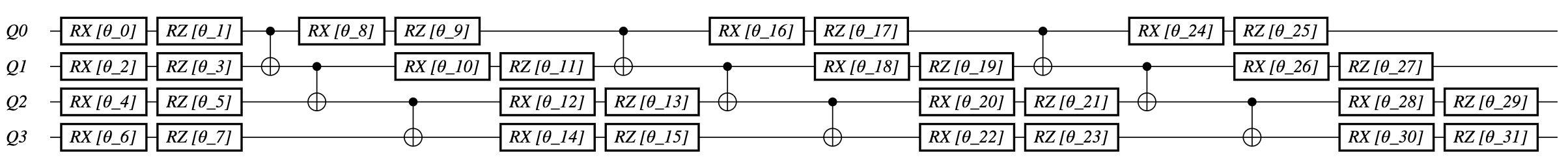
Display
1n_layers = 4
2circ_Linear = HEA_Linear(nqbits, n_layers, [RX,RZ], CNOT)
3circ_Linear.display()
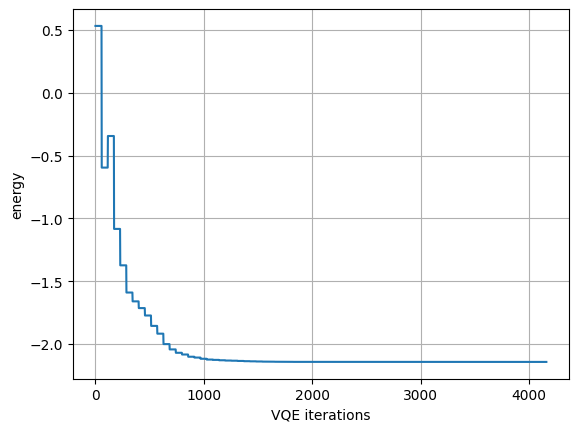
Variational Quantum Eigensolver
 1from qat.plugins import ScipyMinimizePlugin
 2qpu = get_default_qpu()
 3optimizer_scipy = ScipyMinimizePlugin(method="BFGS", # Methods
 4                                      tol=1e-6,
 5                                      options={"maxiter": 200},
 6                                      x0=np.random.rand(n_layers*nqbits))
 7stack1 = optimizer_scipy | qpu
 8
 9import numpy as np
10import matplotlib.pyplot as plt
11
12# construct a (variational) job with the variational circuit and the observable
13job = circ_Linear.to_job(observable=model)
14# we submit the job and print the optimized variational energy (the exact GS energy is -3)
15result1 = stack1.submit(job)
16print(f"Minimum VQE energy ={result1.value}")
17plt.plot(eval(result1.meta_data['optimization_trace']))
18plt.xlabel("VQE iterations")
19plt.ylabel("energy")
20plt.grid()
21plt.savefig("newfigure.pdf")
VQE - Unitary Coupled Cluster
This part is adapted from myQLM documentation demo
The Variational Quantum Eigensolver method solves the following minimization problem: $$ E = \min_{\vec{\theta}}\; \langle \psi(\vec{\theta}) \,|\, \hat{H} \,|\, \psi(\vec{\theta}) \rangle $$
Here, we use a Unitary Coupled Cluster trial state, of the form: $$ |\psi(\vec{\theta})\rangle = e^{\hat{T}(\vec{\theta}) - \hat{T}^\dagger(\vec{\theta})} |0\rangle $$
where $\hat{T}(\theta)$ is the cluster operator: $$ \hat{T}(\vec{\theta}) = \hat{T}_1(\vec{\theta}) + \hat{T}_2(\vec{\theta}) + \cdots $$
where $$ \hat{T}_1 = \sum_{a\in U}\sum_{i \in O} \theta_a^i\, \hat{a}_a^\dagger \hat{a}_i \qquad \hat{T}_2 = \sum_{a>b\in U}\sum_{i>j\in O} \theta_{a, b}^{i, j}\, \hat{a}^\dagger_a \hat{a}^\dagger_b \hat{a}_i \hat{a}_j \qquad \cdots $$
$O$ is the set of occupied orbitals and $U$, the set of unoccupied ones.
 1from qat.fermion.chemistry.pyscf_tools import perform_pyscf_computation
 2
 3geometry = [("H", (0.0, 0.0, 0.0)), ("H", (0.0, 0.0, 0.7414))]
 4basis = "sto-3g"
 5spin = 0
 6charge = 0
 7
 8(
 9    rdm1,
10    orbital_energies,
11    nuclear_repulsion,
12    n_electrons,
13    one_body_integrals,
14    two_body_integrals,
15    info,
16) = perform_pyscf_computation(geometry=geometry, basis=basis, spin=spin, charge=charge, run_fci=True)
17
18print(
19    f" HF energy :  {info['HF']}\n",
20    f"MP2 energy : {info['MP2']}\n",
21    f"FCI energy : {info['FCI']}\n",
22)
23print(f"Number of qubits before active space selection = {rdm1.shape[0] * 2}")
24
25nqbits = rdm1.shape[0] * 2
26print("Number of qubits = ", nqbits)
If we make the plot amongst the HF, MP2 with FCI is the reference we obtain
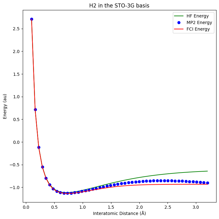
In these such cases, methods like Hartree-Fock (HF) and Møller-Plesset perturbation theory (MP2) become less accurate compared to Full Configuration Interaction (FCI).However in this case for Hydrogen this difference is barely visible, because the HF energy is totally on the same path as FCI from the beginning till the minimum energy point then the curve begins to experience the bond dissociation when the two hydrogen molecules move far each other
Following to show the molecular Hamiltonian
1from qat.fermion.chemistry import MolecularHamiltonian, MoleculeInfo
2
3# Define the molecular hamiltonian
4mol_h = MolecularHamiltonian(one_body_integrals, two_body_integrals, nuclear_repulsion)
5
6print(mol_h)
MolecularHamiltonian(
- constant_coeff : 0.7137539936876182
- integrals shape
- one_body_integrals : (2, 2)
- two_body_integrals : (2, 2, 2, 2) )
Computation of cluster operators $T$ and good guess $\vec{\theta}_0$
We now construct the cluster operators (cluster_ops) defined in the introduction part as $\hat{T}(\vec{\theta})$, as well as a good starting parameter $\vec{\theta}$ (based on the second order Møller-Plesset perturbation theory).
1from qat.fermion.chemistry.ucc import guess_init_params, get_hf_ket, get_cluster_ops
2
3# Computation of the initial parameters
4theta_init = guess_init_params(
5 mol_h.two_body_integrals,
6 n_electrons,
7 orbital_energies,
8)
9
10print(f"List of initial parameters : {theta_init}")
11
12# Define the initial Hartree-Fock state
13ket_hf_init = get_hf_ket(n_electrons, nqbits=nqbits)
14
15# Compute the cluster operators
16cluster_ops = get_cluster_ops(n_electrons, nqbits=nqbits)
17
18
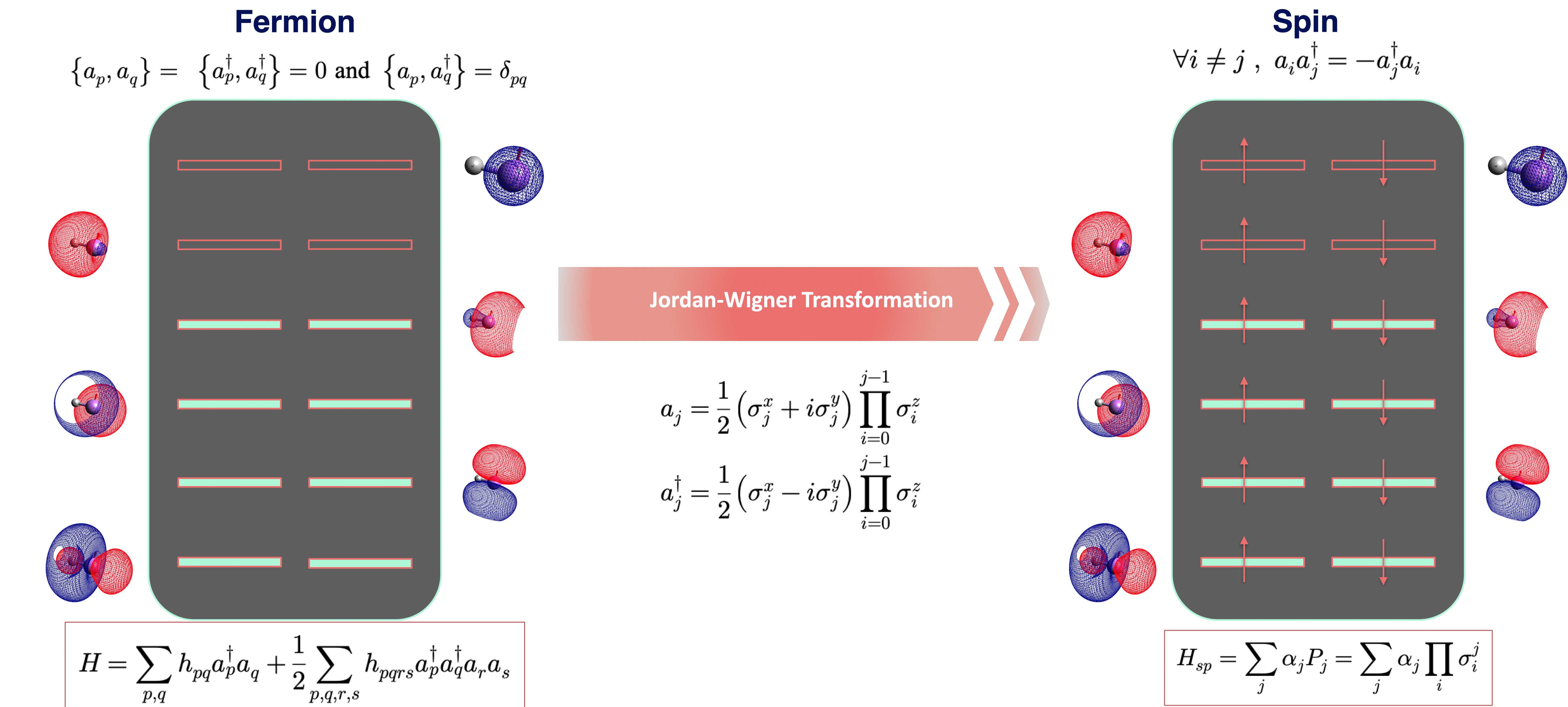
19from qat.fermion.transforms import transform_to_jw_basis # , transform_to_bk_basis, transform_to_parity_basis
20from qat.fermion.transforms import recode_integer, get_jw_code # , get_bk_code, get_parity_code
21
22# Compute the ElectronicStructureHamiltonian
23H = mol_h.get_electronic_hamiltonian()
24
25# Transform the ElectronicStructureHamiltonian into a spin Hamiltonian
26H_sp = transform_to_jw_basis(H)
27
28# Express the cluster operator in spin terms
29cluster_ops_sp = [transform_to_jw_basis(t_o) for t_o in cluster_ops]
30
31# Encoding the initial state to new encoding
32hf_init_sp = recode_integer(ket_hf_init, get_jw_code(H_sp.nbqbits))
33
34print(H_sp)
 1(-0.09886396933545824+0j) * I^4 +
 2(0.16862219158920938+0j) * (ZZ|[0, 1]) +
 3(0.12054482205301799+0j) * (ZZ|[0, 2]) +
 4(0.165867024105892+0j) * (ZZ|[1, 2]) +
 5(0.165867024105892+0j) * (ZZ|[0, 3]) +
 6(0.17119774903432972+0j) * (Z|[0]) +
 7(0.12054482205301799+0j) * (ZZ|[1, 3]) +
 8(0.17119774903432972+0j) * (Z|[1]) +
 9(0.04532220205287398+0j) * (XYYX|[0, 1, 2, 3]) +
10(-0.04532220205287398+0j) * (XXYY|[0, 1, 2, 3]) +
11(-0.04532220205287398+0j) * (YYXX|[0, 1, 2, 3]) +
12(0.04532220205287398+0j) * (YXXY|[0, 1, 2, 3]) +
13(0.17434844185575668+0j) * (ZZ|[2, 3]) +
14(-0.22278593040418448+0j) * (Z|[2]) +
15(-0.22278593040418448+0j) * (Z|[3])
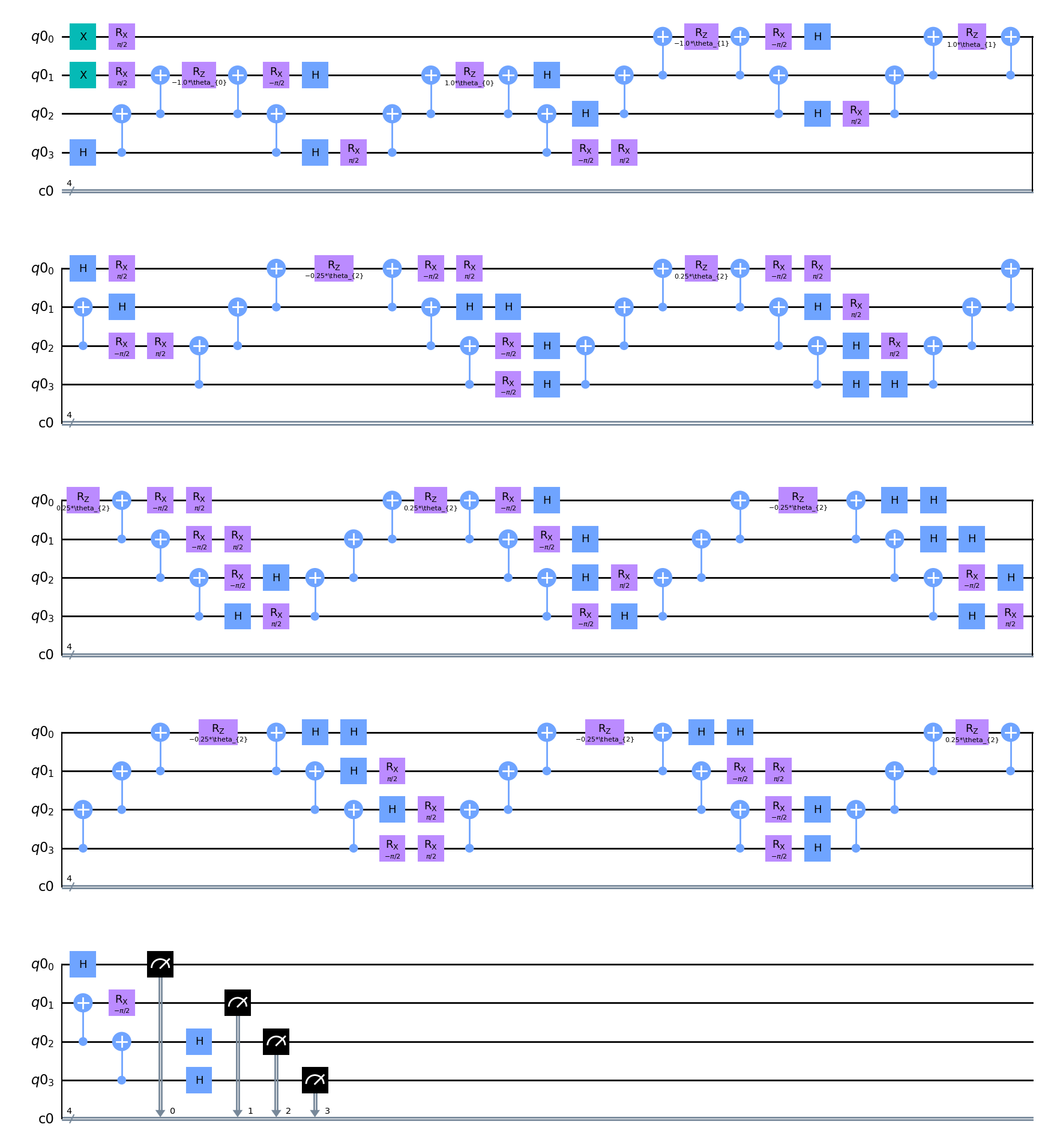
Applying the trotterization method
 1from qat.lang.AQASM import Program, X
 2from qat.fermion.trotterisation import make_trotterisation_routine
 3prog = construct_ucc_ansatz(cluster_ops_sp, hf_init_sp, n_steps=1)
 4
 5prog = Program()
 6reg = prog.qalloc(H_sp.nbqbits)
 7
 8# Initialize the Hartree-Fock state into the Program
 9for j, char in enumerate(format(hf_init_sp, "0" + str(H_sp.nbqbits) + "b")):
10    if char == "1":
11        prog.apply(X, reg[j])
12
13# Define the parameters to optimize
14theta_list = [prog.new_var(float, "\\theta_{%s}" % i) for i in range(len(cluster_ops))]
15
16# Define the parameterized Hamiltonian
17cluster_op = sum([theta * T for theta, T in zip(theta_list, cluster_ops_sp)])
18
19# Trotterize the Hamiltonian (with 1 trotter step)
20qrout = make_trotterisation_routine(cluster_op, n_trotter_steps=1, final_time=1)
21
22prog.apply(qrout, reg)
23circ = prog.to_circ()
24
25prog = construct_ucc_ansatz(cluster_ops_sp, hf_init_sp, n_steps=1)
26circ = prog.to_circ()
27circ.display()
For the molecule $H_2$, it has double qubit excitation and by using the UCC method to simulate on this molecule, I obtain the the circuit construction as bellow with the interprobility with Qiskit and this construction is based on the staire-case algorithms
Using the Gradient Based Optimizer to solve the VQE
The graphic is show:
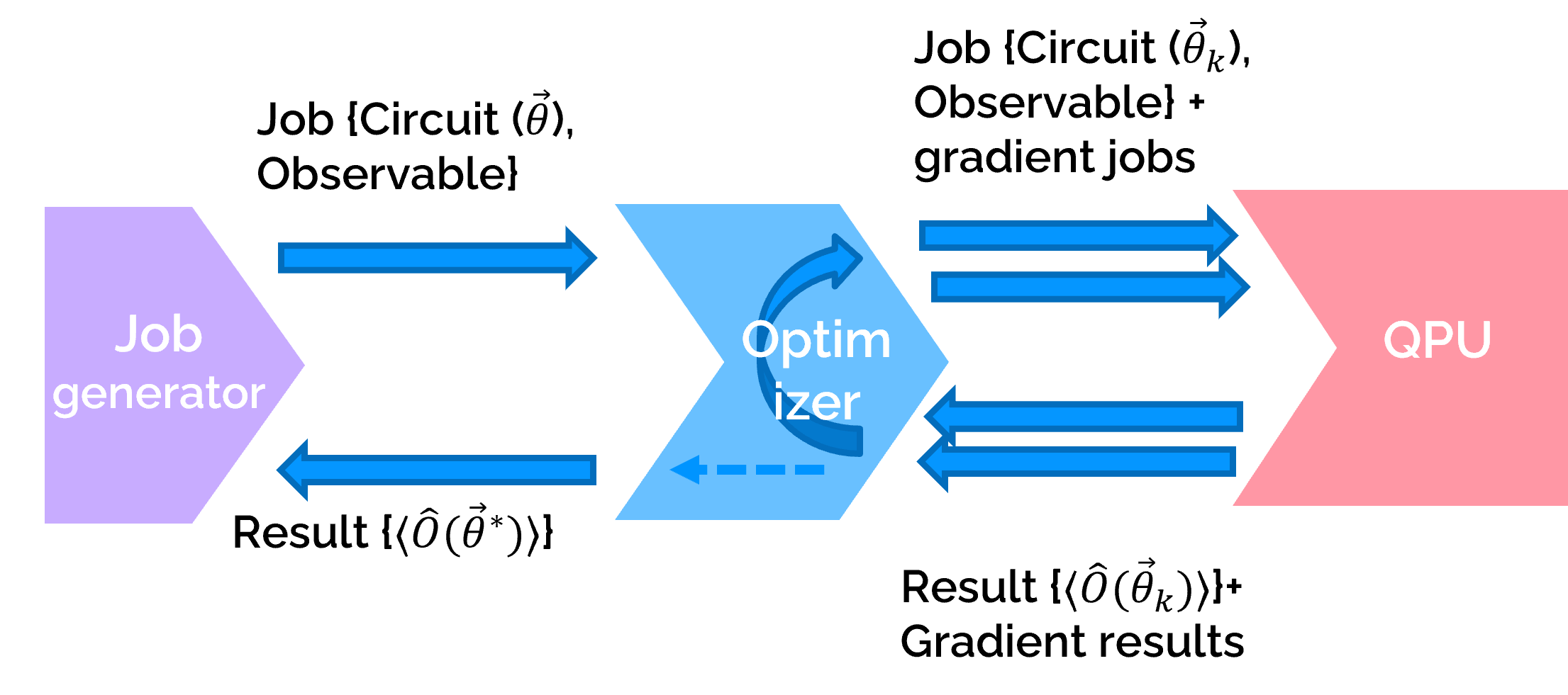
 1job = circ.to_job(observable=H_sp, nbshots=0)
 2
 3from qat.qpus import get_default_qpu
 4from qat.plugins import ScipyMinimizePlugin
 5
 6optimizer_scipy = ScipyMinimizePlugin(method="BFGS", tol=1e-3, options={"maxiter": 1000}, x0=theta_init)
 7qpu = optimizer_scipy | get_default_qpu()
 8result = qpu.submit(job)
 9
10print("Minimum energy =", result.value)
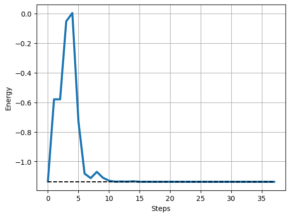
Minimum energy = -1.1372692847285149 \
Make the plot
 1%matplotlib inline
 2import matplotlib.pyplot as plt
 3
 4plt.plot(eval(result.meta_data["optimization_trace"]), lw=3)
 5plt.plot(
 6    [info["FCI"] for _ in enumerate(eval(result.meta_data["optimization_trace"]))],
 7    "--k",
 8    label="FCI",
 9)
10
11plt.xlabel("Steps")
12plt.ylabel("Energy")
13plt.grid()