Estimating Molecular Ground State Energy
Variational Quantum Eigensolver (VQE) using PennyLane
Overview
Variational Quantum Eigensolver (VQE) is a hybrid quantum-classical algorithm used to estimate the ground-state energy of molecular systems. In this tutorial, we demonstrate how to use PennyLane to perform VQE on the Beryllium Hydride (BeH₂) molecule. We start by building the molecular Hamiltonian then prepares a trial wave function, and the classical optimizer adjusts the parameters to minimize the energy.
1. Building the electronic Hamiltonoian
Import necessary libraries
import pennylane as qml
from pennylane import numpy as np
import functools
Define molecular geometry
mol=qml.qchem.mol_data("BeH2")
symbols = ["H","Be","H"]
geometry = np.array([[0.0, 0.0, -1.7],[0.0,0.0,0.0], [0.0, 0.0, 1.7]])
mol1=qml.qchem.mol_data("BeH2")
print(mol1)
(['Be', 'H', 'H'], tensor([[ 4.79404621,  0.29290755,  0.        ],
            [ 3.77945225, -0.29290755,  0.        ],
            [ 5.80882913, -0.29290755,  0.        ]], requires_grad=True))
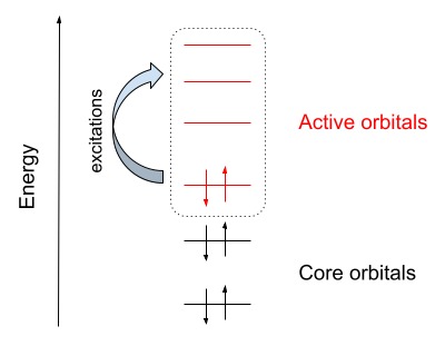
Define active space
Define an active space to perform quantum simulations with a reduced number of qubits by classifying the molecular orbitals as core and active orbitals.
core, active = qml.qchem.active_space(6, 5, active_electrons=4, active_orbitals=3)
print('core orbitals:', core, '\nactive orbitals:', active )
core orbitals: [0]
active orbitals: [1, 2, 3]
Build the Hamiltonian
H, qubits = qml.qchem.molecular_hamiltonian(symbols, geometry, active_electrons=4, active_orbitals=4)
print('qubits:',qubits,'\n\nH =',H)
qubits: 8
H =   (-14.225298300082315) [I0]
+ (-0.017858339631270377) [Z4]
+ (-0.017858339631270377) [Z5]
+ (-0.01785833963125627) [Z7]
+ (-0.01785833963125623) [Z6]
+ (0.18376934404852158) [Z3]
+ (0.1837693440485218) [Z2]
+ (0.189293865627094) [Z0]
+ (0.189293865627094) [Z1]
+ (0.07464706092699114) [Z0 Z2]
+ (0.07464706092699114) [Z1 Z3]
+ (0.0872371502053069) [Z0 Z4]
+ (0.0872371502053069) [Z1 Z5]
+ (0.0872371502053263) [Z0 Z6]
+ (0.0872371502053263) [Z1 Z7]
+ (0.09401471929144516) [Z2 Z4]
+ (0.09401471929144516) [Z3 Z5]
+ (0.09401471929146607) [Z2 Z6]
+ (0.09401471929146607) [Z3 Z7]
+ (0.0942777355550643) [Z4 Z6]
+ (0.0942777355550643) [Z5 Z7]
+ (0.0987691272565404) [Z2 Z5]
+ (0.0987691272565404) [Z3 Z4]
+ (0.09876912725656237) [Z2 Z7]
+ (0.09876912725656237) [Z3 Z6]
+ (0.10034008122331718) [Z4 Z7]
+ (0.10034008122331718) [Z5 Z6]
+ (0.10166582964774823) [Z0 Z5]
+ (0.10166582964774823) [Z1 Z4]
+ (0.10166582964777082) [Z0 Z7]
+ (0.10166582964777082) [Z1 Z6]
+ (0.11246477255979793) [Z4 Z5]
+ (0.11246477255984795) [Z6 Z7]
+ (0.11360615202622484) [Z0 Z1]
+ (0.11637400311980817) [Z0 Z3]
+ (0.11637400311980817) [Z1 Z2]
+ (0.12193472299847673) [Z2 Z3]
+ (-0.04172694219281703) [Y0 Y1 X2 X3]
+ (-0.04172694219281703) [X0 X1 Y2 Y3]
+ (-0.014428679442444536) [Y0 Y1 X6 X7]
+ (-0.014428679442444536) [X0 X1 Y6 Y7]
+ (-0.014428679442441326) [Y0 Y1 X4 X5]
+ (-0.014428679442441326) [X0 X1 Y4 Y5]
+ (-0.006062345668252879) [Y4 Y5 X6 X7]
+ (-0.006062345668252879) [X4 X5 Y6 Y7]
+ (-0.004754407965096297) [Y2 Y3 X6 X7]
+ (-0.004754407965096297) [X2 X3 Y6 Y7]
+ (-0.00475440796509524) [Y2 Y3 X4 X5]
+ (-0.00475440796509524) [X2 X3 Y4 Y5]
+ (0.00475440796509524) [Y2 X3 X4 Y5]
+ (0.00475440796509524) [X2 Y3 Y4 X5]
+ (0.004754407965096297) [Y2 X3 X6 Y7]
+ (0.004754407965096297) [X2 Y3 Y6 X7]
+ (0.006062345668252879) [Y4 X5 X6 Y7]
+ (0.006062345668252879) [X4 Y5 Y6 X7]
+ (0.014428679442441326) [Y0 X1 X4 Y5]
+ (0.014428679442441326) [X0 Y1 Y4 X5]
+ (0.014428679442444536) [Y0 X1 X6 Y7]
+ (0.014428679442444536) [X0 Y1 Y6 X7]
+ (0.04172694219281703) [Y0 X1 X2 Y3]
+ (0.04172694219281703) [X0 Y1 Y2 X3]
charge=0, mult=1, basis='sto-3g', method='dhf', active_electrons=4, active_orbitals=4, mapping='jordan_wigner'
2. Simulation Setup
Define the cost function to compute the expectation value of the molecular Hamiltonian in the trial state prepared by the circuit.
Prepare initial state and ansatz
initial_state = qml.qchem.hf_state(4,qubits)
singles, doubles = qml.qchem.excitations(4, qubits)
s_wires, d_wires = qml.qchem.excitations_to_wires(singles, doubles)
ansatz = functools.partial(qml.UCCSD, init_state=initial_state, s_wires=s_wires, d_wires=d_wires)
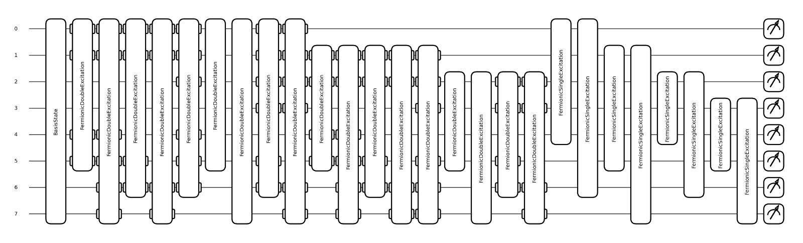
Visualize the circuit
qml.draw_mpl(cost)(np.zeros(len(singles)+len(doubles)))
(<Figure size 3000x900 with 1 Axes>, <Axes: >)
Define the device and cost function
dev = qml.device('lightning.qubit', wires=qubits)
@qml.qnode(dev)
def cost(params):
    ansatz(params, wires=dev.wires)
    return qml.expval(H)
3. Running the VQE Optimization
Now we proceed to minimize the cost function to find the ground state of the $BeH_{2}$ molecule. To start, we need to define the classical optimizer and initialize the circuit parameter $\theta$.
Initialize optimizer and parameters
optimizer = qml.GradientDescentOptimizer(stepsize=0.4)
theta = np.array(np.random.normal(0, np.pi, len(singles) + len(doubles)), requires_grad=True)
print(cost(theta))
-14.54714957820648
Optimization loop
# store the values of the cost function
energy = [cost(theta)]

# store the values of the circuit parameter
angle = [theta]

max_iterations = 80
conv_tol = 1e-06

for n in range(max_iterations):
    theta, prev_energy = optimizer.step_and_cost(cost, theta)

    energy.append(cost(theta))
    angle.append(theta)

    conv = np.abs(energy[-1] - prev_energy)

    if n % 2 == 0:
        print(f"Step = {n},  Energy = {energy[-1]:.8f} Ha")

    if conv <= conv_tol:
        break

print("\n" f"Final value of the ground-state energy = {energy[-1]:.8f} Ha")
#print("\n" f"Optimal value of the circuit parameter = {angle[-1]:.4f}")
Step = 0,  Energy = -14.63557759 Ha
Step = 2,  Energy = -14.78225259 Ha
Step = 4,  Energy = -14.88670434 Ha
Step = 6,  Energy = -14.95791760 Ha
Step = 8,  Energy = -15.00763932 Ha
Step = 10,  Energy = -15.04499395 Ha
Step = 12,  Energy = -15.07580596 Ha
Step = 14,  Energy = -15.10340072 Ha
Step = 16,  Energy = -15.12944838 Ha
Step = 18,  Energy = -15.15456471 Ha
Step = 20,  Energy = -15.17872483 Ha
Step = 22,  Energy = -15.20157124 Ha
Step = 24,  Energy = -15.22265201 Ha
Step = 26,  Energy = -15.24158903 Ha
Step = 28,  Energy = -15.25816881 Ha
Step = 30,  Energy = -15.27236184 Ha
Step = 32,  Energy = -15.28429206 Ha
Step = 34,  Energy = -15.29418402 Ha
Step = 36,  Energy = -15.30230986 Ha
Step = 38,  Energy = -15.30894833 Ha
Step = 40,  Energy = -15.31435887 Ha
Step = 42,  Energy = -15.31876880 Ha
Step = 44,  Energy = -15.32236951 Ha
Step = 46,  Energy = -15.32531797 Ha
Step = 48,  Energy = -15.32774085 Ha
Step = 50,  Energy = -15.32973939 Ha
Step = 52,  Energy = -15.33139419 Ha
Step = 54,  Energy = -15.33276939 Ha
Step = 56,  Energy = -15.33391611 Ha
Step = 58,  Energy = -15.33487528 Ha
Step = 60,  Energy = -15.33567983 Ha
Step = 62,  Energy = -15.33635639 Ha
Step = 64,  Energy = -15.33692662 Ha
Step = 66,  Energy = -15.33740823 Ha
Step = 68,  Energy = -15.33781579 Ha
Step = 70,  Energy = -15.33816130 Ha
Step = 72,  Energy = -15.33845473 Ha
Step = 74,  Energy = -15.33870437 Ha
Step = 76,  Energy = -15.33891713 Ha
Step = 78,  Energy = -15.33909878 Ha

Final value of the ground-state energy = -15.33917949 Ha
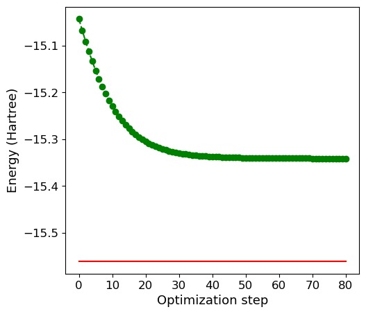
4. Visualization of the Optimization Process
Plot energy convergence
import matplotlib.pyplot as plt

fig = plt.figure()
fig.set_figheight(5)
fig.set_figwidth(12)

# Full configuration interaction (FCI) energy computed classically
E_fci = -15.56089
ax1 = fig.add_subplot(121)
ax1.plot(range(n + 2), energy, "go", ls="dashed")
ax1.plot(range(n + 2), np.full(n + 2, E_fci), color="red")
ax1.set_xlabel("Optimization step", fontsize=13)
ax1.set_ylabel("Energy (Hartree)", fontsize=13)
plt.xticks(fontsize=12)
plt.yticks(fontsize=12)
plt.show()
References
- Peruzzo et al., A variational eigenvalue solver on a photonic quantum processor, Nat. Commun. 5, 4213 (2014).
- Seeley, Richard & Love, The Bravyi–Kitaev transformation, J. Chem. Phys. 137, 224109 (2012).
- Cao et al., Quantum Chemistry in the Age of Quantum Computing, Chem. Rev. 119, 10856–10915 (2019).
- Born & Oppenheimer, Quantum Theory of the Molecules, Ann. Phys. 84, 457 (1927).
- Seeger & Pople, Self-consistent molecular orbital methods XVIII, J. Chem. Phys. 66, 3045 (1977).
- Fermann & Valeev, Fundamentals of Molecular Integrals Evaluation, arXiv:2007.12057.
- Bao et al., Automatic Selection of an Active Space, J. Chem. Theory Comput. 14, 2017 (2018).
- PennyLane Tutorial: VQE Demo — https://pennylane.ai/qml/demos/tutorial_vqe